Are you intending to train your own RAVE model on a dedicated machine with SSH? This tutorial is made for you!

In this article, we will explain how to

1. install RAVE on a computer / remote server
2. choose & preprocess a dataset
3. choose the good configuration
4. monitor the training
5. export the model for RAVE VST / nn~.

Warning: this tutorial does not explain how to train RAVE on unofficial Google Colab notebooks, like this one by Moisés Horta.

Preparing the training

Prerequisites

What you need to train a model is :

• a computer / server with a GPU of at least 8GB (5Gb for raspberry) for the full time of training, with SSH access. You can check the minimum GPU memory required for a given RAVE architecture in the README.
• a dataset of at least one hour. If you don't have, go fetch one on websites like Kaggle, or generate synthetic data with frameworks like pyo.

Warning: The duration of a full RAVE training is difficult to hard to predict exactly, as it depends of the chosen configuration, the data, and your machine. Usually, first training phase last for about three or four days, and second phase may take from four days to three weeks.

Install Python through miniconda

Here, will see how to install all the required dependencies needed on an empty Linux server, such as the one you can rent online on platforms such as vast.ai. If you want to train it on your own computer or server, the installation is the same ; however, you may encounter some specific problems because of the current internal state of your machine (dependencies, bash profiles, etc...). In case of problems, do not hesitate to make a clean pass on your machine !

Note 1 : On Windows, you will have to install GitBash as a terminal interface to follow this tutorial. <br/> Note 2 : Some online GPU servers propose to start from Docker images with PyTorch installed, such that you may not need to follow some of the steps below.

In this tutorial we will use miniconda as a python package manager, that install a minimal framework allow to safely create Python environements. Download miniconda on the webpage, and install it on your platform.

# prepare folder for miniconda at root folder (called ~)
mkdir -p ~/miniconda3
# Download miniconda (for Linux)
wget https://repo.anaconda.com/miniconda/Miniconda3-latest-Linux-x86_64.sh -O ~/miniconda3/miniconda.sh
# Download miniconda (for Windows)
wget https://repo.anaconda.com/miniconda/Miniconda3-latest-Linux-x86_64.sh -O ~/miniconda3/miniconda.sh
# install miniconda
bash ~/miniconda3/miniconda.sh -b -u -p ~/miniconda3
rm -rf ~/miniconda3/miniconda.sh
# init miniconda
~/miniconda3/bin/conda init bash
~/miniconda3/bin/conda init zsh
# close and start again your terminal, or launch the following command
cd ~
source .bashrc

miniconda should be installed now ; you can verify it by seeing a (base) indication at the very left of your command prompt, as in the image below.

Install Python environment

miniconda is used to create Python environement, that are very useful to make sure that a given application won't messup the requirements of the others. For example, you can check the current location of your python envionrment :

which python 
# should return sth like YOUR_MINICONDA_PATH/bin/python

that is, when the (base) environment is activated, it will use the default python executable of miniconda. We will now create an environment specific to RAVE :

# create environment
conda create -n RAVE python=3.9
# activate environment
conda activate RAVE 
which python 
# should return sth like YOUR_MINICONDA_PATH/envs/RAVE/bin/python

If your RAVE environment has been activated properly, you should see a (RAVE) indication instead of (base) at the very left of your command prompt. By using which, we can see the python executable of our environement has changed : our dependencies are then isolated from other applications, and will not mess around!

<img src="assets/article_3/environment_ok.png"/>

Now we created our environement, we will then download the RAVE git repository, and install RAVE and its required dependencies :

which pip
# should return sth like YOUR_MINICONDA_PATH/envs/RAVE/bin/pip
pip install acids-rave

we download the RAVE repository with git, and install the requirements with python package manager pip (we check it's the one of our environment before). The installation of the RAVE requirements may take some time but will be finised after that, so it's the good moment to take care of the dataset.

Data preparation

The training dataset needs to be preprocessed before being usable for a RAVE training. It is difficult to elaborate precise guidelines on what could be a good dataset or not, but some criteria are mandatory for the model to be trained accurately :

• amount of data - the more data you have, the more the model will be able to understand the underlying properties of your dataset.
• homogeneity - if your dataset comprises very different types of sounds, the model may struggle to learn everything and to gather everything ; however, if the dataset is too similar, the model may fall into a low-capacity behavior with a very low variety. For example, a dataset with a single instrument with various playing styles is usually a good choice, as it is both various and constrained in the kind of sounds it gathers. Similarly, training on music samples of a given musical genre will provide enough diversity to the model to generalize well, but also to find common variations that it will be able to generate during inference.
• audio quality - of course, if your sounds have a low audio quality, or very noisy, this will make the training procedure more difficult. You should also consider the overall dynamics of your dataset : if some sounds are much louder than others, it will generally be learned in a better way that sounds with a lower amplitude. If needed, you may consider to make a compression / normalization pass on your overall dataset, in order to help the model to generate these sounds more accurately.

Here, we will use the musicnet dataset, contaning 330 freely-licensed classical music recordings. All the audio sounds must be placed in a specific folder, and be pre-processed with the rave preprocess command :

rave preprocess --input_path /path/to/your/dataset --output_path /target/path/of/preprocessed/files --channels 1

We can indicate the number of channels with the --channels keyword :

• if we want our model to generate mono signals, write --channels 1
• if we desired a stereo model, write --channels 2
• for a quadriphonic model --channels 4.
• ...

However, only mono models are compatible with RAVE VST, so we will train a monophonic models with --channels 1. Now, let’s launch this command and wait for the preprocessing to be done. Once preprocessing has been finished, there should be two files in the output directory of your preprocessing :

cd /target/path/of/preprocessed/files
ls
# > data.mdb      metadata.yaml
cat metadata.yaml
du -sh data.mdb

the data.mdb file contains the compressed data that was just pre-processed, and metadata.yaml contains some information about your dataset.

Pro-tip: you can add the --lazy mode data preprocessing, that uses ffmpeg in real-time during tranining. This avoids data duplication in an other folder, but also slows down data import during training. Use it if you have a really really big dataset!

Training your model

RAVE has been installed, and the data is ready. We are now able to start our training!

Detaching your process

Before starting your training, we will have to make sure that our training does not stop when will we close the terminal window. Indeed, when you launch a command on the terminal, the process is said to be attached to your command window : it implies that when you close the window, you close the process. We will then have to detach the process from the window ; on Linux, we will here use screen, but you could also use tmux or other.

# If your machine is fresh, you could not have it installed by default
sudo apt install screen
# We make a screen called train_musicnet
screen -S train_musicnet

You should see a cleaned window ; you can think of it as a tab in a browser, that you activated in parallel to the window you were before. With screen, you can detach the current window with Ctrl+A, then D : you should go back to the previous window. Now, if you close the terminal window and go back, all the commands you would have launched in the train_musicnet window would not be affected!

You can see the list of screen with the -ls keyword ; let's go back in the screen where we will start the training, and activate our RAVE environment.

# display possible screens
screen -ls
# re-attach train_musicnet
screen -r train_musicnet
conda activate RAVE

Training the model

Now is the big time : we will start the training process! There are a lot of possible options, that you can display by using the --help keyword, that will list all possible keywords for the train command. For this training we will launch the following command, that we will describe keyword by keyword.

rave train --help
# [...] every train keyword [...]
rave train --name musicnet --db_path /path/to/dataset --out_path /path/to/model/out --config v3 --config noise --augment mute --augment compress --augment gain --save_every_epoch 100000

where you have to replace /path/to/dataset by your dataset path, and /path/to/model/out by the directory where you want your model to be saved in. Here is the description of the keywords we chose :

• --name is the name of your training ; you can choose it arbitrarily
• --db_path is the directory of your preprocessed data
• --out_pathis the output directory of for you model and the training monitoring
• --config is specifying the model configuration, by default v2. You can add additional configurations by putting more than one --config keyword ; more precisions below.
• --augment is adding data augmentations to the model ; more precisions below.
• --save_every_epoch saves the trained model every X epochs ; handy to resume later specific checkpoints of the model.

Choosing the architecture. The choice of the model architecture is the most important decision when training a model. The main configuration are the one listed under the Architecture type of the config table in RAVE official README, that we show again just below :

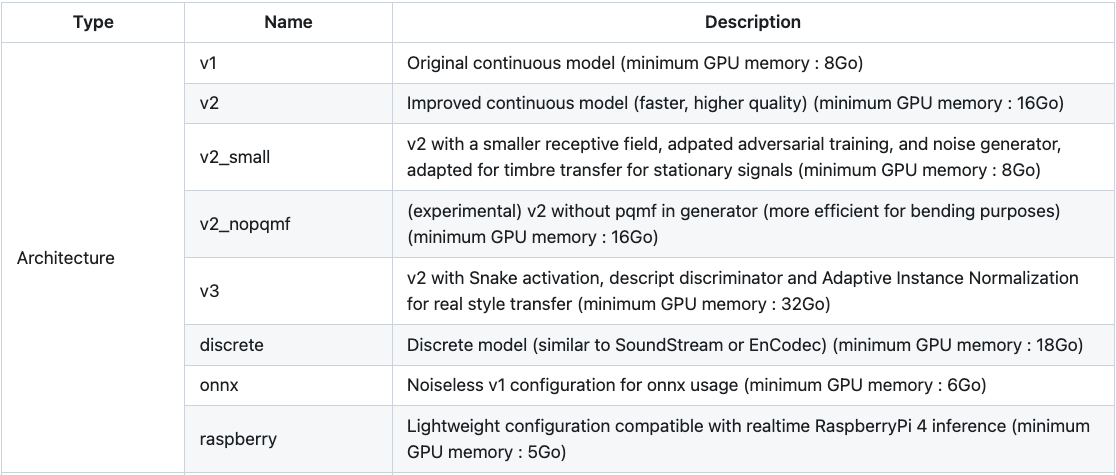
While this choice is arbitrary, here some tips to select wisely the configuration you need.

• if your dataset is composed of simple, or short sounds such as instrument samples, single voices, or sound fx, and you want the model to perform timbre transfer, we advise you to use either v1 or v2_small. These configurations are lighter, and more suitable for sounds that are not very complex.
• if your dataset is composed of layered music, or complex sounds, we advise you to use either v2, v3, or discrete configuration. If you want to use RAVE as a synthesizer by directly controlling the latent varaibles, do not use the discrete configuration ; however, if you plan to train a prior using msprior, use the discrete configuration.
• if you want to use your model on a raspberry pi, select the raspberry configuration. This configuration is not able to learn complex sounds though, so choose your dataset wisely.

Regularization options. With v2 configuration, some additional regularization options are available. Regularization has an impact on how the model build its latent space, thus on how the sounds are organized in the latent parameters. Regularization strategies can also affect the output quality. Quoting again the config table in RAVE official README :

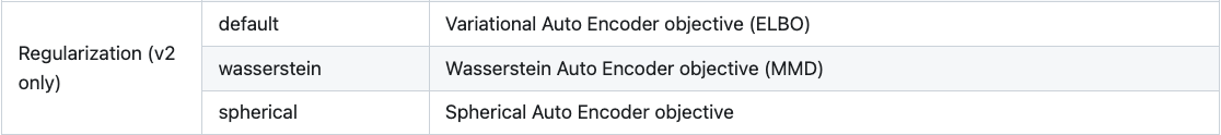
• default is the classic regularization term used for variational auto-encoders, used by default. Use this one before any further experiment!
• wasserstein is a regularization term inspired by optimal transport ; it may provide better reconstruction results, at the price of a more messy latent space (no smoothness in latent exploration, for example)
• spherical enforces the latent space to be distributed on a sphere. It is experimental, do not try that first!

Additional options. Last but not least, some very important options are availble in the Others section of the config table in RAVE official README : 

• causal: enforces the model to only use the past samples of the incoming waveform. In real-time setups, this will reduce the perceived latency of the model ; however, reconstruction quality will be lower.
• noise: adds a noise synthesizer to the RAVE's decoder ; may be important for learning of sounds with important noisy components.
• hybrid: replaces the input of the encoder by a mel representation of the incoming signal ; may be interesting for learning on voice.

Choosing augmentations. The --augment keyword can be used to add data augmentations in your training process, that can be very important in case of small datasets. Data augmentations perform randomly signal operations on the data at training data, allowing to virtually increase the diversity of the dataset. Three data augmentations are so far available:

• mute allows to randomly silence out incoming batches, enforcing your model to learn silence if your dataset does not contain any
• compress randomly applies small amount of compression, allowing the model to be trained on dynamical modifications of your sounds
• gain randomly applies gain (by default between -6 and 3 dB) to the incoming data, allowing the model to be trained on different amplitudes of your sounds

Do not hesitate to try them out, especially if your dataset is small!

Lanching the training. Once you chose your training configuration, everything is setup! Just launch your command and, once the training status bar appears, you're all good! You can detach the process, and start monitoring your training.

Note: If your training fails at some point for some reason, you can resume the last saved state of your training by using the -ckpt checkpoint :

rave train [...your previous training args...] --ckpt /path/to/model/out

and RAVE will automatically detect the last saved checkpoint of your training. If you want to restart from a specific checkpoint, you can write the full path to your .ckpt file :

rave train [...your previous training args...] --ckpt /path/to/model/out/version_X/checkpoints/model_XXXXX.ckpt

Monitoring your training

Connecting to tensorboard

You can monitor your training using tensorboard, a very useful tool that allows to display several metrics about the current training state, as well as some sound samples. To do this, make another screen (or tmux) and launch the tensorboard command in the root of your training output directory :

screen -S monitor 
conda activate RAVE
cd /path/to/model/out
tensorboard --logdir . --port XXXX

where you replace XXXX by a four-numbered port of your choice. tensorboard, at some point, should give you an address ; if the training is on your computer, you can directly copy and past the given address to your favorite browser. However, if you are using SSH protocol, you will have to bridge the port you gave with the ssh port you connect on. You can redirect a port with the -L keyword ; for exemple, by connecting to your server with

ssh your/ssh/address -L 8080:localhost:8080

by putting XXXX in the tensorboard command to 8080, you should be able to connect on your local network with the 127.0.0.1:8080 address on your browser.

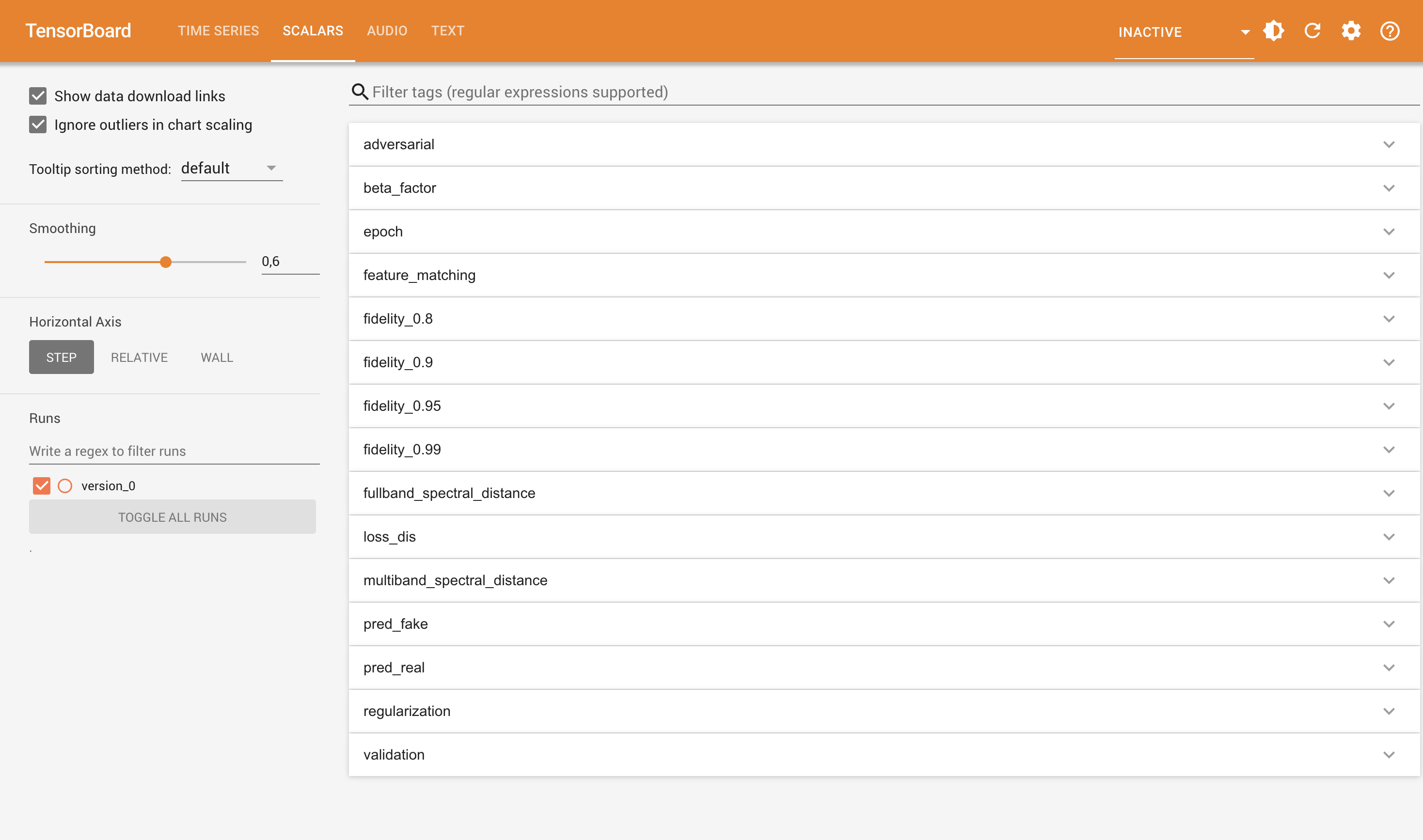
Monitoring metrics

Tensorboard has a Scalars tab, where you are able to monitor diverse current metrics of your training. First, be aware that RAVE's training process has two distinct phases :

• phase 1 : auto-encoding phase - The encoder and the decoder of the model are trained jointly on a spectral loss ;
• phase 2 : adversarial phase - The encoder is frozen and a discriminator is introduced ; the decoder is fine-tuned with the discriminator using an adversarial training setup.

The duration of the first phase is defined by the chosen configuration, but is 1 million batch most of the time.

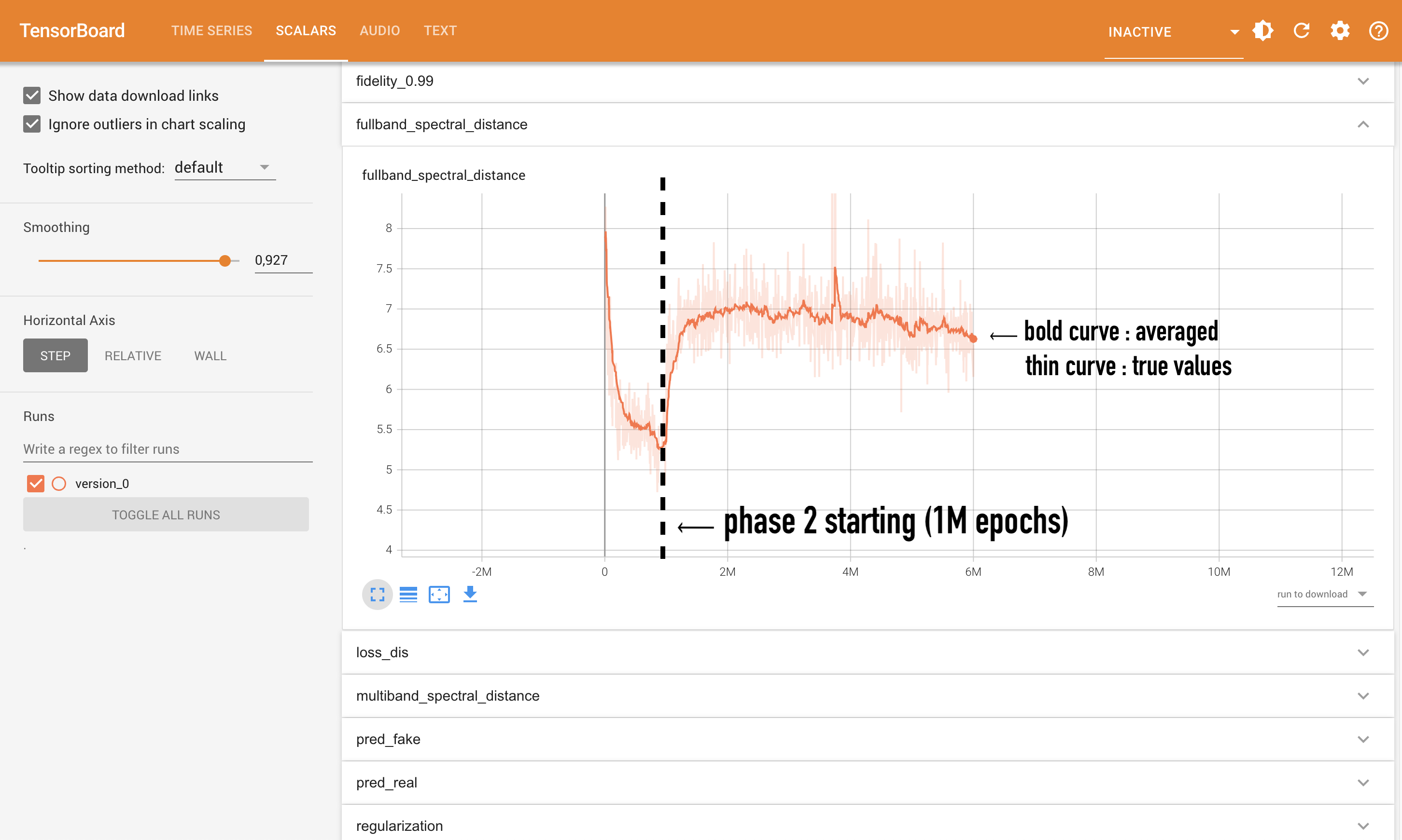
Monitoring phase 1. The encoder and the decoder are trained using three losses : the fullband_spectral_distance and multiband_spectral_distance, and regularization. Typically, the two first losses should be regularaly decreasing during this first phase. Losses are plotted by batch, so the curves may be be a little noisy ; do not hesitate to play with the smoothness parameter at the left to see the averaged evolution of your loss.

The regularization loss is an additional term that influences the shape of your latent space. The meaning of this loss depends on the choses regularization strategy in the configuration :

• with default regularization, this regularization term is the difference between the latent space and an isotropic gaussian. A zero regularization typically means that your latent space is random noise, a degenerated behaviour. Reversely, a very high regularization term means that your latent space is very "rough", or bursted around undesirable values.
• with wasserstein, this regularization term evaluates how much your latent space ressembles an unit open ball. The difference with the previous one is that it only prevents latent parameters to be very far from this ball, but does not penalize the "roughness" of the latent space. This can help the model to reconstruct accurately the input sound, but also to put very different data nearby in the latent space ; be careful if you plan to manipulate latent variables manually.
• with spherical, there is no regularization term : latent projections are forced to lie on a multi-dimensional sphere.

Besides the training loss, another important metrics for this phase 1 are the latent_pca phases. You should have four of these plots, named latent_pca with a following float number. This plot is an indicator of the latent topology of the model : it is the number of dimensions for a PCA to explain out X% of your dataset's variability, where X is the number after the curve's name. More concretely, let's take the following curve :

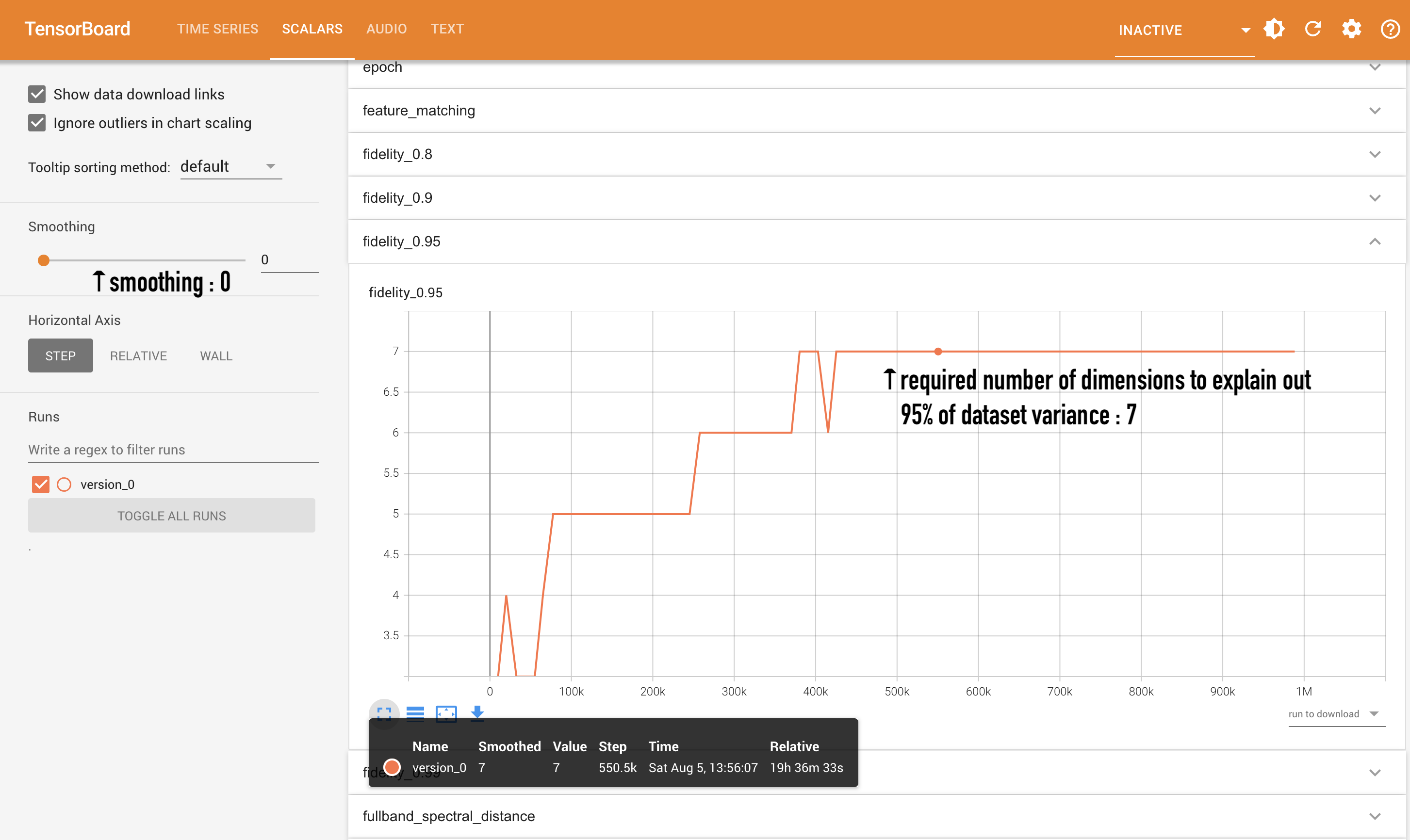
it means that your model needs X dimensions out of 128 to represent 95% of your dataset after dimensionality reduction. Given that RAVE performs the same kind of dimensionality reduction at export, it will also indicate you the number of the dimensions that you will be able to control (by default ; see below). These curves are very useful to obtain some insights about your latent space's diversity : typically, if your dataset is very complex and your model only needs 2 dimensions to explain it out, there might be something wrong with your training. Note that, however, this critierion is very loose ; don't be too anxious about it.

Monitoring phase 2. The training drastically changes during phase 2 : adversarial training comes into play!

Adversarial training is typically hard to monitor, so let's explain things out a bit. Adversarial training is based on a generator and a discriminator, that are trained in a concurrent way : the discriminator is trained to separate the generator's output to the real data, and the generator is trained to fool it. As training goes by, the discriminator should be able to detect synthesized sound more and more accurately, and thus the generator to synthesize more and more accurate data.

Adversarial training is a very efficient training scheme, but may be very unstable and is difficult to monitor : indeed, the adversarial loss is not indicating at all if the model has been accurately trained, but rather the balance between the discriminator and the generator. Hence, if the discriminator has a very little loss (it detects every time the synthesized data), it can mean that the generator is very very bad, or discriminator very very powerful (and reversely).

Typically, the spectral losses used in phase 1 will suddenly jump ; do not worry, this is a normal behavior, as the introduction of the discriminator in the training process is perturbing the system a little bit. Once your model has reached phase 2, you should be able to monitor new losses in your tensorboard: adversarial, pred_fake, pred_real, loss_dis, and feature_matching.

• adversarial is the adversarial loss of the model's decoder : a low value means that the decoder manages to fool the discriminator.
• loss_dis is the adversarial loss of the model's discriminator : a low value means that the discriminator separates accurately real from synthesized data.
• pred_real and pred_fake show the centroid of respectively the real and synthesized data in the last layer's embedding of the discriminator. The discriminator is typically trained to separate both in a binary way ; hence, these centroids are trained to be very separated.
• feature_matching is an additional term used by the generator to help it match the real data statistics within discriminator's internal layers. This help is double-edged though : if the discriminator is bad, so will be this loss.

When should I stop the training?

Listen to your sounds! Adversarial training is very difficult to monitor, especially with audio where mathematimatical distances may be very far away from the actual perceived quality, the best is simply to listen to reconstructions. For this, go into the Audio tab of the tensorboard, and listen to the audio_val samples. The audio extract will make you hear, consecutively, the original and the reconstructed sound. If your target audio has several channels, they will be unfolded to be also placed consecutively. The reconstructed samples come from the validation set, meaning that they were not part of the training data : this is helping to also evaluate the generalization abilities of your model.

Under-fitting vs. over-fitting. In generative machine learning, we teach models to reproduce a given set of data. In tasks such as recognition or classification, we typically want our models to perform with unknown data as well as with training data : if we want to distinguish meowing sounds from barking sounds, we do not want an alarm behind to mislead our model. To this end, a good practise is to retrieve a little bit of data from our training set, and evaluate our model regularly on this unseen data. As neural models are very powerful, they are very prone to a phenomenon called over-fitting : fitting so much the data that they may be over-sensible to trivial details, and then failing to perform correctly on unseen data. The opposite is, without any suspense, under-fitting : the model performs quite poorly, but with similar results on seen and unseen data.

With some machine learning tasks, we then observe how our model performs with unseen data, and stop training as soon as the model start to overfit. However, things are a little different in generative learning : we aim to model a given distribution. In some applications generative modelling should be able to model unknown data, such as neural codecs. In some tasks though, such as timbre transfer, the objective is not so clear : overfitting would not prevent a creative use, it can be quite the opposite. However, in-domain over-fitting may be a good measure of your model's steadiness : for example, if you model violin sounds, and that your model fails drastically at re-generating them, it may indicate that your training went wrong as it means that the model's internal representation is degenerated. This can be observed by observating the validation loss on the tensorboard : typically, if you observe repetitive spikes and unstable evolution, it can mean that it is time to stop training your model.

Starting again from phase 2. Phase 2 may be particularly unstable, and its performance may depend on the chosen architecture, but also to the nature of your sounds. You may start again from a checkpoint (using --ckpt, see above) that finished the phase 1 to override some adversarial parameters. For example, adjusting the update periodicity of the discriminator can help if the discriminator struggles to differentiate real from synthetic data : to do that, re-start your training by adding --override "model.RAVE.update_discriminator_every = 4"to your command. To access all the parameters of your training, you can check the config.gin at the root of your model's output directory.

Exporting the model

You're happy with your model? Time to export it! To do that, use the rave export command :

rave export --run path/to/model --name your_model_name --output /path/to/save/exported/model --streaming True

Let's explain a little bit of these options.

• --run indicates the path of your model checkpoint. You can put the base folder, a specific version, or a specific .ckpt file.
• --name is the name of the exported model ; it is arbitrary, name it like you want!
• --output is the output directory of the exported model ; by default, it will be placed in the --run folder.
• --streaming is very important : put it to True if you're planning to use the model with nn~ or RAVE VST! If you don't your model will be clicking, as the convolution layers will not cache the streamed data.

At the end, you should have your scripted model (with .ts extension) in the output path. That's all!

Setting model's dimensionality. Some additional options are available to set up manually the number of controllable dimensions : this will influence, for example, the amount of dimensions of encode and decode functions in nn~. There are two ways to set up the number of dimensions :

• --fidelity : automatically finds the number of dimensions to explain out the given amount of data in the latent space (with PCA, see above). For example, giving --fidelity 0.98 will retrieve the number of latent dimensions required to explain 98% of the dataset variance.
• --latent_size : sets a fixed amount of accessible latent dimensions. For example, --latent_size 8 will enforce 8 latent inputs / outputs in nn~, whatever the dataset variance it describes.

Well, that's it! If you encounter bugs during training, do not hesitate to put an issue on the RAVE github, or to find some help among other users on the RAVE discord. Keep in touch!